Your Step-By-Step Guide for Performance-Level Calculations of Safety-Critical Electronics

Table of Content

1. Introduction

If you are a designer of an electronic system and you need to understand how well your system reacts to a state that can cause harm to a human being (a battery pack catching fire due to cell overvoltage or cell over temperature), it is useful to calculate a “Performance Level”.

This guide will help you develop an understanding of

What are performance-level calculations?

Why and where are they needed?

The prerequisite steps and calculations needed to attain Performance-level calculations.

This guide will take into example a battery-management system for performing and explaining performance level calculations. The guide first introduces the metrics used and then uses Siemens Norms (SN-29500) and ISO-13849 for performing Performance Level calculations.

Performance Level is mostly also used and accepted when you certify your system for multiple UL standards such as UL2580, UL2271, and UL1973. In each of these standards, a section called Functional Safety is detailed. Different FUSA standards can be used to prove that your system complies with a level of functional safety. In this guide, we have detailed the use of ISO-13849 and have used that to calculate a Performance level for our system.

If you use an industrial norm such as Siemens SN-29500 standard, you would need to purchase the corresponding documentation as that will be the basis for FIT calculations that lead to the Performance Level calculations. It is also recommended to purchase ISO-13849. ISO-13849 is the basis on which all understandings about performance level calculations are performed.

1.1 Performance Level

“Performance Level” is a performance metric that provides insight into a control system’s ability to detect conditions that may lead to a catastrophic failure or that can create a hazardous situation for humans. In the case of battery-management systems, an example of catastrophic failure would be the batteries catching fire due to over-charging / short-circuiting.

Performance levels (PL) is a metric that is applied to different safety-related aspects in a complete system. The performance grading is performed on a scale from “a” to “e”. PLe (Performance Level e) is the best performance level attainable and PLa is the worst. This rating helps provide the manufacturer with important information ascertaining what part of the SRP/CS (Safety Related Part of a Control System) system needs improvement.

PL (Performance Level) is calculated using a multistep process that involves calculating the FIT (Failure in Time) for each component you have in the system. Before delving into PL (Performance Level) calculations, we need to talk about these two terms; FIT (Failure in Time) and MTTF (Mean Time to Failure).

1.2 FIT (Failure In Time) and MTTF (Mean Time To Failure)

FIT (Failure in Time) is a measure of the reliability of the component and how it will perform and can also help you identify the components in your design that are most prone to failure! Components with moving mechanical parts such as relays, switches, etc. are usually more prone to failures, and have therefore a high value of FIT, depicting that they may fail more often in each period.

FIT and MTTF are two terms used to provide an estimation of how many times a component fails in a specified period for specific operating conditions. A third term MTBF (Mean Time Between Failures) is also a popular metric, but it usually applies to repairable systems. MTTF applies to systems that must be replaced and cannot be repaired.

FIT is a metric that denotes the number of failures in 1×10⁹ hours. MTTF and FIT are directly related to each other, in the following relation:

MTTF = 1×10⁹/ FIT

For example, a FIT of 5 would have an MTTF of 2×10⁸ hours. An MTTF of 2×10⁸ hours means that the component would have been in operation for 2×10⁸ hours before a failure occurred. A FIT of 5 means that the component is likely to fail 5 times in 1×10⁹ (1 billion) hours of operation.

All reliability estimates are based on a well-defined standard such as MIL-HDBK-217 or Siemens SN-29500. These form the basis for calculations performed and the FIT values calculated. A good way to get a basic understanding of FIT can be to use MTBF (Mean Time Between Failure) calculators like Ram Commander (the MTBF calculator is a small part of it) and ItemSoft (which can import BOMs and perform batch calculations). Using these tools requires some knowledge of the standard, therefore, it is helpful to spend some time reading the relevant documentation of the standards used.

To read more about FIT, MTTF, and MTBF, you can read our blog.

1.3 Difference Between Performance Level and FIT (Failure in Time) Calculations

Performing a FIT (Failure in Time) analysis for your system is different than calculating performance levels. A performance level is performed only on the components that relate to the safety (hazard prevention) related aspects of the system and no other features. For example, a BJT circuit that simply turns on a status LED is not part of the performance level analysis but can be part of your FIT analysis.

1.4 Introduction to System Categories, Safety Functions, and Safety Blocks

ISO 13849-1 assigns a system into 1 (or more) of 4 categories that are used to define your system. The document details the definitions and methodologies of calculating PL and deciding other details such as what category your system will belong to.

The ISO-13849 standard documentation should be studied extensively to come to an understanding of your exact requirements and what category your system belongs to. For a basic understanding of what this category means, we can look at the following image:

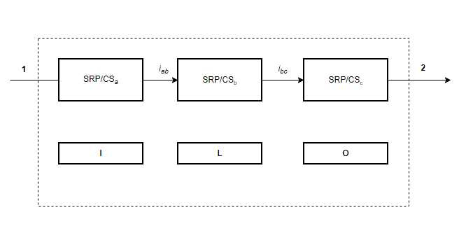
Figure 1a (Image: Oxeltech)

The above diagram category defines the assignment of major system components into basic categories. Input, Logic, and Output.

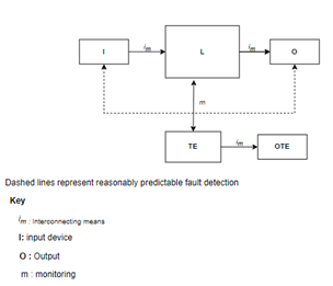
Figure 1b (Image: Oxeltech)

Depicted above is a category 4 architecture. It has the following blocks:

Input: All components that contribute to an input must fall into the input block.

Logic: All components that make a logical decision based on available data (along with supporting components) lie in this block.

Output: All components that are driven by the Logic block are added to this block. Only components that directly prevent a hazardous state will be added here. The Logic block decides whether to drive these components.

TE (Test Equipment): This Block consists of parts that act as redundancy to your main Input/Logic/Output Blocks. These can be used to test the system independently of the main blocks.

OTE (Output Test Equipment): This Block consists of components that are actuated if any component in the TE block goes into a failure state. For e.g., If the system is measuring system pack voltage in the Input Block by adding up the cell voltages, then the TE block can measure the entire pack voltage using a separate pack voltage sensor.

The various blocks defined above have different purposes that will be explained in greater detail in Chapter 3.

The block diagrams shown above will then be assigned to different safety functions. Each safety function might have 1 or more block diagrams (depending on the system size). A sample safety function is shown in the image below. This is an over-current safety function and gives you a basic idea about the blocks used to create the block diagram for the safety function.

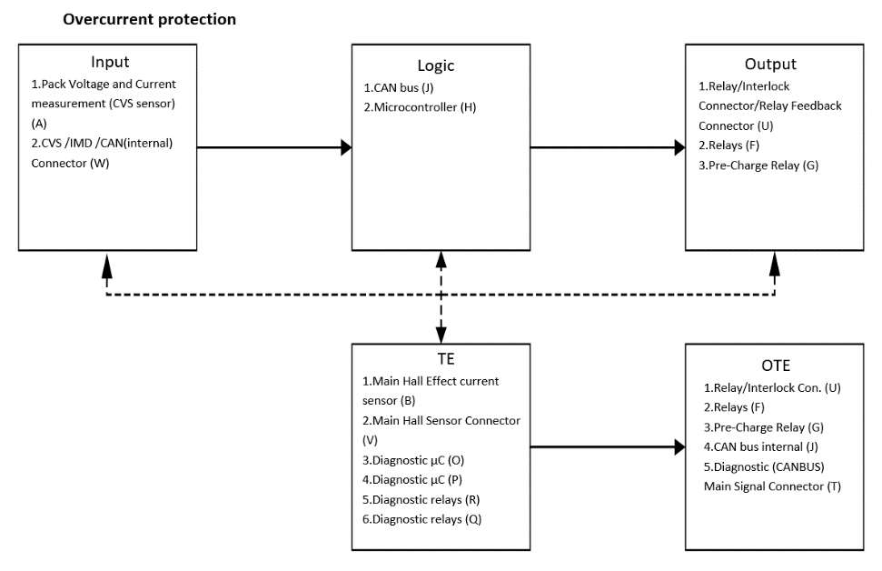
Figure 1c (Image: Oxeltech)

2. How to Calculate FIT (Using SN29500)

2.1 Introduction to the basic terminology used in SN29500

Ambient Temperature: The ambient temperature refers to the temperature of the immediate surroundings of the component when it is not in operation.

Mean Ambient Temperature: The mean ambient temperature represents the average value of the ambient temperature experienced by components in similar applications. This may involve considering temperature fluctuations over time.

Reference Conditions: The reference conditions specified in this standard’s individual parts are chosen to align with most applications for the mentioned components. These conditions serve as a basis for expected values.

Operating mode: The operating mode description indicates whether the components are continuously operated or if there are breaks during their application. The following distinctions are made:

Description of Environment: The description of the operating environment outlines the prevailing climatic and mechanical stresses that occur during the component’s operation.

Continuous duty:

Relatively long duration with a constant load (e.g., process controls).
Relatively long duration with a changing load (e.g., telephone switching equipment).
Relatively long duration with a constant minimum load and short-duration maximum loads (e.g., fire-alarm systems).

Intermittent duty:

Constant load during the operating phases (e.g., process controls).
Changing load during the operating phases (e.g., control units in machining installations, road traffic signals).

2.2 Calculation Methodology / Example

The primary factor used in determining reliability for sub-assemblies and equipment units is the failure rate. Siemens AG utilizes the component failure rates specified in the standard SN29500, as a consistent foundation for reliability predictions. This standard also includes the specific conditions under which the component failure rates are applicable (known as reference conditions). Reference conditions are essential when stating failure rates or comparing values from different sources. The IEC 61709 serves as the basis for defining the reference conditions and conversion models that account for failure rates under varying stress conditions. The stress models outlined in this standard are used as the foundation for converting failure rate data from reference conditions to actual operating conditions.

For an overview, the SN29500 standard uses the following method to estimate the reliability:

Figure 2 (Image: Oxeltech)

The Reference FIT refers to the FIT value that a component of a particular category is estimated to have at any time. The Operating FIT refers to the FIT value when a component is tested at operating conditions. On the contrary, the stress profile is an accelerated testing for the component where a component is under stress.

Overall, you will need to know the base reference FIT which will then be converted to the operating FIT. The result is a FIT that is appropriate for your desired conditions. These operating conditions should not be more than the absolute maximum ratings. The reference conditions for most of the components are mentioned in the standard document for all component categories.

2.2.1 Calculating FIT for a Single Component

To calculate the FIT (Failures in Time) of a component, you can follow the steps outlined below:

Identify the specific type of component you are working with, such as a passive component, discrete semiconductor, or integrated circuit.
Refer to the appropriate Siemens norm for that component type, such as SN29500-1, SN29500-2, SN29500-3, and so on. For example, if you are working with a passive component, you would refer to SN29500-4. The Figure below shows the norm number for each category:

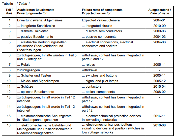
Figure 3 (Image: SN29500 documentation)

Study the norm document corresponding to the identified norm number. Look for the specific formulas provided for the component category you are dealing with. These formulas will help you calculate the FIT.
Within the norm, identify the component category and note the reference FIT value mentioned for that category. This reference FIT value serves as a baseline for further calculations.
Calculate the operating FIT (λ) based on the reference FIT (λ_ref). To do this, refer to the formulas provided in the norm document and consult any accompanying tables or information. Consider dependencies such as temperature dependence (πT) and voltage dependence (πU), which may be listed in tables.
Use the identified formulas and relevant dependencies to calculate the operating FIT for the specific component you are analyzing.

Let’s calculate the FIT for C1901 in the following sample BOM.

Figure 4 (Image: Oxeltech)

As in Figure 4, the “Part” (extension) for passive components is 4, so we will refer to SN29500-4. Once you read the document, you can conclude that the following assumptions are made for the calculation:

Operating Voltage: For capacitors 50 % of the rated voltage, if not otherwise stated.

Mean Ambient Temperature: 40°C for all passive components

After the assumptions, you will find the table for capacitor failure rates as shown in Figure 6

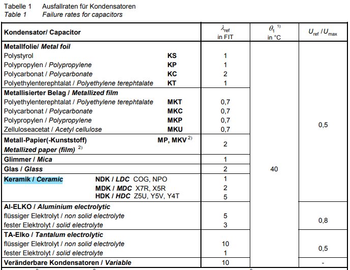
Figure 5 (Image: SN29500 documentation)

As given in the BOM, the C1901 capacitor is a ceramic capacitor with the temperature coefficient X7R, following information can be concluded for the component from the table.

Reference FIT (λ_ref) = 2

Reference Capacitor Temperature (Θ1) = 40°C

The ratio of Reference Voltage to Maximum Voltage (U_ref/_Umax) = 0.5

Now that you have the reference FIT, you need to find the formula to calculate operating FIT. The formula for capacitors is given as:

Figure 6 (Image: SN29500 documentation)

To calculate λ, you need π_T, π_U, & π_Q which are temperature dependence, voltage dependence, and quality factor respectively. The formula for each of these is given or as an alternative, lookup tables are also provided. You can either refer to tables that implement that formula or directly use the formula. Once you know the value of π_T, π_U, & π_Q, multiply each dependency and get the value of λ. we will use tables to get the value.

Calculating πu_,

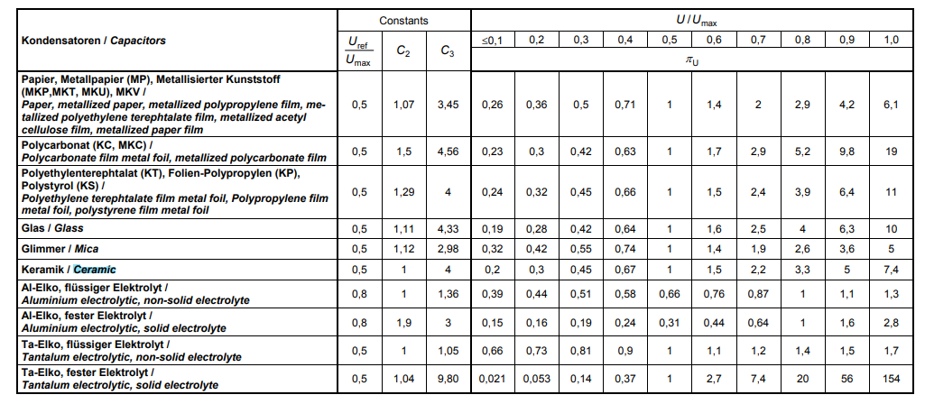
Figure 7 (Image: SN29500 documentation)

As shown in Figure 8, the π_U, for the ceramic capacitor goes from 0.2 to 7.4 based on the ratio of operating voltage to the max voltage. Given that we consider the value of U/U_max to be 0.2, π_U is 0.3.

Calculating π_T,

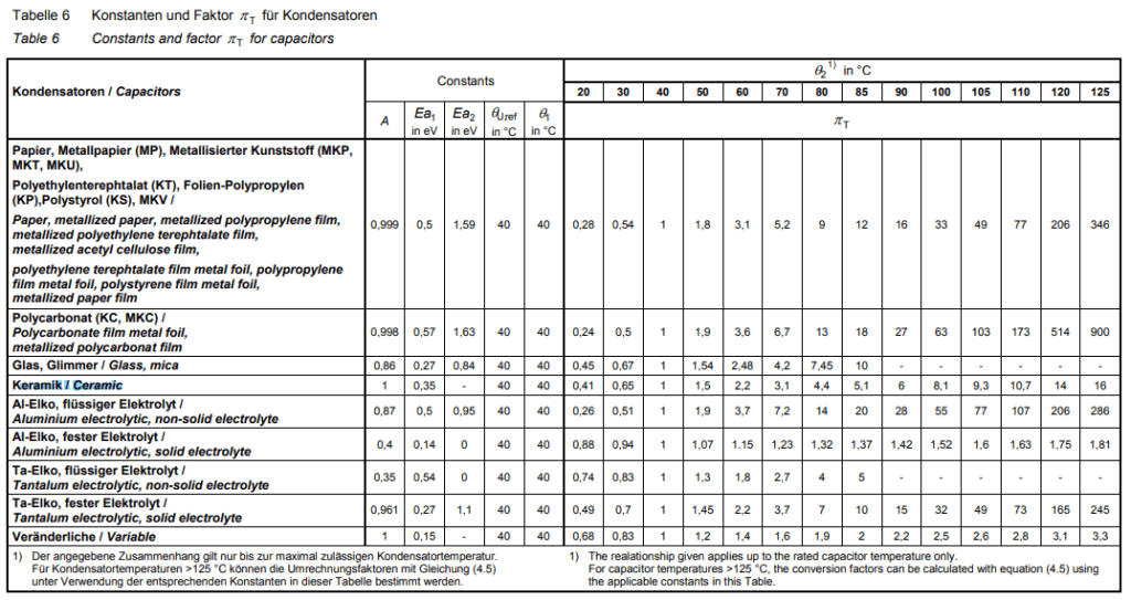
Figure 8 (Image: SN29500 documentation)

As shown in Figure 9, the π_Tfor the capacitor goes from 0.41 to 16 based on the actual capacitor temperature (Θ2). Considering an actual temperature of 60 °C, the π_Tis 2.2.

Please note that in the formulae, temperature values are always used in Kelvin, so don’t forget to convert your operating temperatures respectively!

Calculating π_Q,

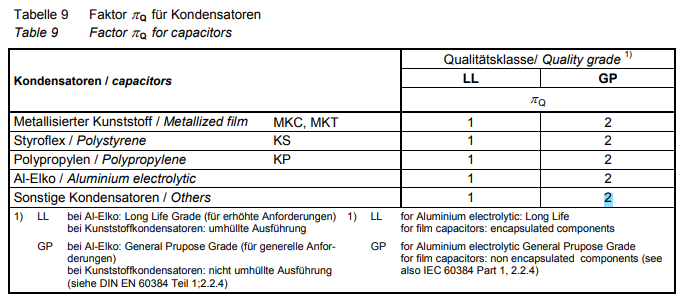
Figure 9 (Image: SN29500 documentation)

Based on the categories, the general-purpose capacitor has a π_Q of 2.

Therefore, the λ can be given as 2*0.3*2.2*2 = 2.64

This value you have calculated is your FIT for that specific component.

2.2.2 Calculating FIT for the Whole System

Above we have calculated the FIT for a single component. Use the same methodology for all components of your system.

Once you have FIT values for all components on 1 single board, you can simply add the relevant FIT values to calculate the overall FIT for the board. You can analyze each FIT value to gain an understanding of what component has the worst FIT (if that is your goal).

Some of the components on your board might not be included in any safety channel. Therefore, we do not have to calculate the FIT of all the components. The complete board FIT is only used when all components of the board are a part of the FIT channel.

In the next part, we will present the safety functions we developed for our board and how it helped to predict the performance level.

3. Performance Level

3.1 Introduction to Safety Channels and Safety Functions

Safety Blocks and Safety functions are two distinct parts of the performance level analysis. Safety Functions are the different indexes on which a system is analyzed. Examples of these are under-voltage protection, overvoltage protection, etc. Each safety function relates to a specific feature or system state that you want to check the performance level for.

Safety Blocks on the other hand is a division of your components. This division simplifies the assignment of components into the safety functions. Each Safety Block has an FIT assigned which is merely the sum of the FIT for all components that make up that block.

3.2 Safety Channels

Safety blocks are the division of your entire system into smaller segments. These smaller segments can then be assigned to the input/logic/output blocks as discussed before. Each block will have an FIT value which is a sum of the relevant FIT’s of components that are assigned to it. A detailed analysis of the schematics in your system is necessary to understand and analyze the components and understand where they fit into your safety blocks.

For example, in the safety functions, the microcontroller will be part of the logic block and the microcontroller will end up being part of a safety block. Let’s call this block “MCU”. The “MCU” safety block will include all components that are relevant to the functioning of the Microcontroller. For example, all decoupling capacitors on the MCU supply pins and all the MCU external oscillators will be part of the safety block.

Another example is the voltage sense circuit for a system that measures voltages using a battery management system IC. The BMS IC will be part of the input block and can be assigned to a safety block. This safety block we could, for example, call “Cell Voltages Sense”.

In Figure 11 below, a sample safety block definition has been listed. These blocks are defined with the characters “A to Y” based on the system we were analyzing. Each block was named and defined by the type of components it consists of. The figure represents the blocks we have defined, and the relevant block FIT we have calculated for them.

Note: There can be external components that are not on the PCBs themselves. You can find their FIT values separately and then assign these FIT values to the respective block these components belong.

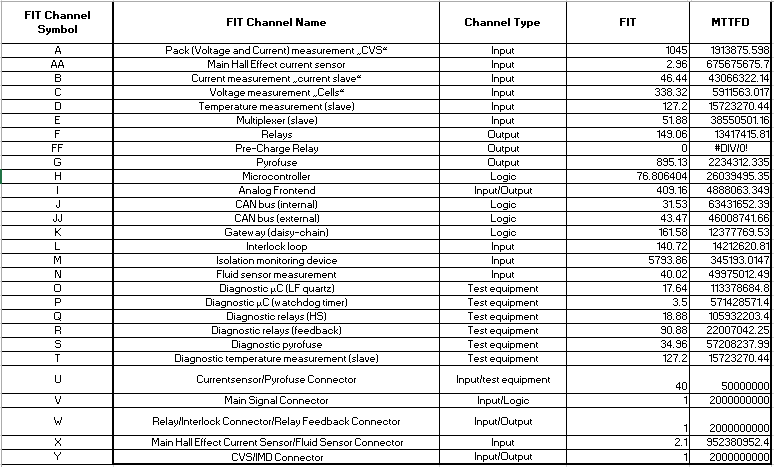
Figure 10 (Image: Oxeltech)

Each block has a specific number of components for which the FIT is calculated in the same way as described in the previous section. The FIT’s of all components in a particular block are summed to get a single FIT for the block itself (number of failures in 1×10⁹ (1 billion) hours). The relevance of the component to that block is understood by understanding how that component works. For example, if we select the “CAN bus (internal)” block J. The FIT for this block will be made up by adding the FIT’s of the following components:

CAN-BUS transceiver IC (through which all data will flow).

Filter Capacitors on the IC supply voltage.

Termination Resistances.

Connectors solely dedicated to the use of CAN BUS.

3.3 Safety Functions

The safety functions are the key metrics on which you will judge the safety-related hazardous states that your system might attain. These states are defined keeping in mind the context of the system. So, sample safety functions can be Over-voltage protection, Short-circuit protection, Over-temperature protection, etc. All the examples listed are actual states that a BMS with Lithium Ion Cells can attain. These can be hazardous to the end user and the surrounding environment as well.

Each safety function can and usually does have multiple safety blocks assigned to it. The assignment of blocks depends on its relevance to that safety function. For example, the “Voltage measurement cells” block C is highly relevant to the safety function “Over-Voltage Protection”. But the “Fluid sensor Measurement” block N has no relevance to the same “Over-Voltage Protection” safety function. By using the relevance of each block, you need to carefully assign your blocks to the relevant safety function architecture diagram.

Let’s now look at the following block diagram representation of how the safety blocks will fit into the safety function block diagram architecture.

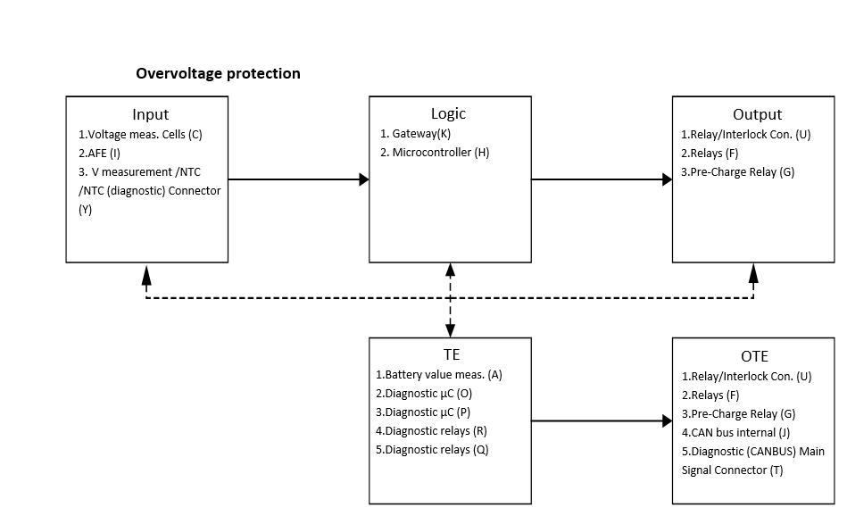
Figure 11 (Image Courtesy: Oxeltech)

The architecture above depicts different inputs, logic, and outputs. A description has been added explaining what components go into each of the blocks:

Input:

1. Voltage meas. Cells (C)

This block contains all components measuring the cell voltages. V Sense resistances, V Sense Filters, and other components that only measure voltages make up this block.

2. AFE (I)

This block contains a BMS IC, and associated resistors and capacitors needed to power and keep the IC in operation. It has other tasks as well (balancing), so it needs a separate block.

3. V measurement /NTC /NTC (diagnostic) Connector (Y)

This block contains a connector needed for cell Voltage Measurement.

Logic:

1. Gateway(K)

This block contains the transceiver and connectors needed for communication between different BMS IC’s. (This BMS IC has daisy chain support)

2. Microcontroller (H)

This block contains the Microcontroller and all associated circuits needed to keep it functional.

Output:

1. Relay/Interlock Con. (U)

This block contains the Relay Connector.

2. Relays (F)

This block contains the 2 Main Series Relays. These are not on the PCB itself, but their FIT is necessary for the PL!

3. Pre-Charge Relay (G)

This Pre-charge is used only when the battery pack is connected to a sink (Motor Drive) for the first time. (There can be instances where the output and the input of the pack are at different potentials. This pre-charge relay coupled with a series resistance is supposed to reduce the surge current.)

Some readers will notice that in the system described above, there is no mention of measuring the safety or calculating the performance level for the high-voltage to low-voltage DC-DC power converters in the system. In fact, the system we are analyzing here is designed in such a way that in the absence of 12V/5V/3.3V, all main relays will open their contacts (these relays are loaded on the Normally Open contacts (N.O.)). This ensures that in the case of a power failure, the system presents no hazard to the operator at all as all N.O. contacts will remain open! That is why the DC-DC power supplies on any PCB are not part of the Performance Level Analysis. You may perform an FIT analysis to provide a reliability estimate for your power supply but finding PL is not necessary (at least for our system). Your system may vary, so you should have a detailed understanding of how your system behaves in various operating conditions!

In the diagram above, the TE block and OTE block will both function as redundancies to the main input, logic, and output blocks. If the cell voltages are within the desired range, but the battery pack voltage is not in the correct range then the control system will activate the relays to disable the system to prevent a hazardous state (function of the TE+OTE).

Using the above block diagram, we add up the FITs of each of the input, logic, and output blocks. We then convert this value into the MTTF (Mean Time to Failure). This MTTF value is the complete sum for this safety function and will be used in the next step.

Let’s assume that from the above-mentioned 28 safety blocks, we made 13 safety functions. Each safety function uses more than one safety block. The FIT for the safety function was the sum of the FIT’s of all safety blocks it included. This was later used to calculate MTTF using the formula (MTTF=1000000000/FIT).

Using the MTTF, the MTTFD was also calculated. MTTFD is the total number of dangerous failures. MTTF and MTTFD are related by the equation:

MTTD=2*MTTF

MTTFD is important in the next step as it allows us to calculate the PFh values.

Figure 13 (Image: Oxeltech)

Once we have defined all block diagrams for each of the safety functions and all safety blocks have their FIT values calculated, we can move on to the Diagnostic Coverage part of the calculations.

3.4 Diagnostic Coverage

The diagnostic coverage average or DC average is a measure of how much weightage a particular safety block has on the entire safety function itself. ISO 13849-1 defines DC as: “The measure of the effectiveness of diagnostics, which may be determined as the ratio between the failure rate of detected dangerous failures and the failure rate of total dangerous failures.”

The formula for the DC average uses DC values which are assigned to each safety block. The value for each safety block is assigned by studying ISO 13849-1. Table E.1 in the ISO standard defines how DC values are assigned to each block (depending on the relevance). Once DC values are assigned to each block, we can then utilize the following formulae to calculate the DC average for the entire safety function.

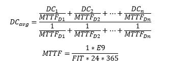
In the above DC average formula, MTTFD (Mean Time to Dangerous Failure) is obtained by using the conversion method for FIT to MTTF and then from MTTF to MTTFD. MTTF and MTTFD are both measured in hours.

For our board, we calculated the DC average for each safety function by first calculating the MTTFD for each block. Then we assigned DC values to each block using the ISO-13849 document. The figure below shows a sample DC value assigned to each block.

Figure 14 (Image Source: Oxeltech)

The table above also shows a Diagnostic Measure assigned to each block. This Diagnostic measure is the action that the software of your controller will perform to independently verify the measurement of an input device. It is an important design feature of your system to have redundancies in your measurement systems. And it is equally important to check those redundant measurements so if you have a difference in the measured values, your system can shut down as one of those measurements is wrong!

Once we have assigned DC values to each safety block, we calculate a DC average value for each safety function. This will be calculated by the formula:

Inputting values into the above equation will give us a DC average for that safety function. In the example, we use the 7 DC values for each safety block that was relevant to the safety function “Under-Voltage Protection”.

Then we input the MTTFD1 – MTTFD7 values. MTTFDn and MTTF are not the same and the “D” indicates that it is the number of dangerous failures (as calculated before). So, the MTTFD1 and DC1 are both supposed to be from the same safety block.

MTTF_D = 2 * MTTF (Estimation that 50% of the failures are dangerous)

MTTF_D is simply the number of dangerous failures which is two times the MTTF of the safety function.

Figure 15 (Image Source: Oxeltech)

Once we have a DC average value for each of the safety functions, we use the following table to check if our DC average for each safety function is high, medium, or low. For our under-voltage protection safety function example shown below, the DC average is 96.2 which is a Medium DC average.

Figure 16 (Image Source: ISO-13849)

3.5 Analyzing Performance Level

Once done with the DC averages, we can move to the final part which is finding out what performance level our safety function lies at. To come to this metric, we use the DC average and the PFH (Probability of Failure per Hour) values. PFH is calculated by:

PFH = 1/ MTTF_D

MTTF_D = 2 * MTTF (Estimation that 50% of the failures are dangerous)

We calculated our PFh values earlier in this guide. PFh is a simple inversion of the MTTFD.

The performance level can be visualized and understood by the following images. The table below uses PFH and the DCavg as the deciding factor for performance levels. The category we selected for our system is 2 which narrows down things a bit.

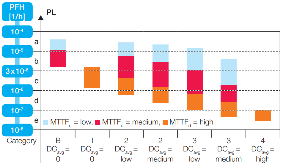
Figure 17 (image source: ISO-13849)

The below table can also be used to directly visualize what PL your system is cohering to. You use the PFH value you calculated earlier to find what Performance Level your safety function has achieved. For example, if the PFH you have calculated is 2×10^-6, then according to Figure 18 below, your safety function has a PLc. A PLc is a good performance level (better than PLa and PLb) and as explained earlier, the higher the PL, the better the performance level of the safety function. The below image is simply the tabular form of Figure 17 without the effect of category.

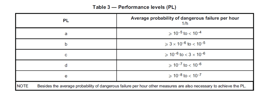
Figure 18 (image source: ISO-13849)

Figure 19 below represents the calculations we performed for estimating PL for our safety functions. The table shows data calculated by using the above process. The safety function “Over-voltage Protection” we were looking at earlier has a resulting Performance Level of “c”. This is an excellent result. If your system analysis results in components that have a poor PL, by improving the components that make up your safety function, you can improve the performance level.

Figure 19 (Image source: Oxeltech)

Once you have calculated the performance level for all your safety functions you have completed the overall process. However, based on the performance level you get, measures can be taken to improve the performance of the overall system. Nevertheless, these different performance levels for our system are advantageous for multiple reasons. Not only does this PL level assist you if you want to get the system certified by UL, but in the process, you have also successfully calculated FIT’s for all components in your schematics. You can now analyze each part in your system and replace those with a high failure rate!